'Analogies Explained' ... Explained
This post aims to present a `less math, more intuition’ overview of Analogies Explained: Towards Understanding Word Embeddings (ICML, 2019, Best Paper, hon mention), following the conference presentation. Target audience: ML, NLP, CL. [Skip to result]
Background
Word Embeddings
Word embeddings $\mathbf{w}=[w^{(1)}, w^{(2)}, … , w^{(d)}]$ are numerical vector representations of words (e.g. $\mathbf{w}_{\text{cat}}=[0.02, 0.29, …, -0.34])$, where each component $w^{(i)}$ can be thought of as capturing a semantic or syntactic feature of the word, and the full vector $\mathbf{w}$ acts as co-ordinates for the word in a high-dimensional “semantic space”.
Word embeddings can be created as a list of word co-occurrence statistics (or their low-rank factorisation); or learned by a neural network, such as Word2Vec (W2V), GloVe or a large language model. We shall see that these are closely related, and that the latter neural word embeddings learn statistics implied by the training algorithm, rather than them being explicitly defined.
Neural word embeddings (or simply embeddings) are useful across a wide variety of tasks involving natural language, from identifying word similarity or grammatical role, to assessing the sentiment in a customer review. Here, we focus specifically on word embeddings learned by Word2Vec and GloVe as the relative simplicity of their training algorithm and model architevture allows rigorous analysis.
Analogies
An intriguing property observed in trained word embeddings is that analogies are often solved simply by adding/subtracting them, e.g.:
“man is to king as woman is to queen”
can be solved using word embeddings by finding that closest to \(\mathbf{w}_{king}-\mathbf{w}_{man}+\mathbf{w}_{woman}\) (omitting $man$, $woman$ and $king$ themselves), which often turns out to be \(\mathbf{w}_{queen}\). This suggests that:
\[\begin{equation} \mathbf{w}_{king} - \mathbf{w}_{man} + \mathbf{w}_{woman} \approx \mathbf{w}_{queen}\, \tag{1}\label{eq:one} \end{equation}\]or, in geometric terms, that word embeddings of analogies approximately form parallelograms:
.
While this seems intuitive, the fact that semantic relationships between words appear as geometric relationships between word embeddings is intriguing since word embeddings are not trained to achieve it! In practice, the parallelograms formed by word embeddings of analogies are not perfect:
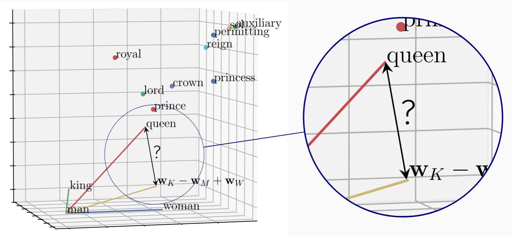
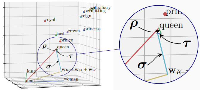
This shows the (exact) parallelogram formed by \(\mathbf{w}_{king}, \mathbf{w}_{man}, \mathbf{w}_{woman}\) and a fourth vertex (\(\mathbf{w}_{king} {\small-} \mathbf{w}_{man} {\small+} \mathbf{w}_{woman}\)) in the $xy$-plane with several word embeddings plotted relative to it. We see that (i) the embedding of $queen$ is not at the fourth vertex, but is the closest embedding to it; and (ii) that embeddings of related words, e.g. \(prince\) and \(lord\), are close relative to random words.
| To explain the relationship between word embeddings of analogies \eqref{eq:one}, we describe the gap (marked ‘?’) between \(\mathbf{w}_{queen}\) and \(\mathbf{w}_{king} {\small-} \mathbf{w}_{man} {\small+} \mathbf{w}_{woman}\); and show that it is small, often smallest, for the word that we expect to complete the analogy. |
We begin by considering what W2V embeddings learn.
Word2Vec
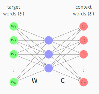
W2V (SkipGram with negative sampling) generates word embeddings by training the weights of a 2-layer “neural network” to predict context words \(c_j\) (i.e. words that fall within a context window of fixed size \(l\)) around each word \(w_i\) (the target word) over a text corpus.
To reduce the computational cost of computing \(p(c_j\!\mid\! w_i)\) over all \(c_j\) in a dictionary \(\mathcal{E}\) using a softmax function, sigmoid functions were trained to classify truly occurring context words from words chosen at random (negative samples).
Levy & Goldberg (2014) showed that under this regime, matrices \(\mathbf{W}, \mathbf{C}\) (whose columns are word embeddings \(\mathbf{w}_i, \mathbf{c}_j\)) approximately factorise a matrix of shifted Pointwise Mutual Information (PMI):
\[\begin{equation} \mathbf{W}^\top\mathbf{C} \approx \textbf{PMI} - \log k\ , \end{equation}\]where $k$ is the chosen number of negative samples and \(\begin{equation} \textbf{PMI}_{i,j} = \text{PMI}(w_i, c_j) = \log\tfrac{p(w_i,\, c_j)}{p(w_i)p(c_j)} \end{equation}\,.\)
The shift $\log k$ is an arbitary artifact of the algorithm, which we address in the paper (Sec 5.5, 6.8) but drop here to simplify. The resulting relationship \(\mathbf{W}^\top\!\mathbf{C} \!\approx\! \textbf{PMI}\) implies that an embedding \(\mathbf{w}_i\) can be seen as a low-dimensional projection of \(\text{PMI}_i\), the $i^{th}$ row of the PMI matrix, or PMI vector.
Proving the embedding relationship of analogies
This suggests observed additive relationships between word embeddings \eqref{eq:one} follow if the projection from PMI vectors to word embeddings induced by the loss function is sufficiently linear and if equivalent relationships exists between PMI vectors, i.e.
\[\begin{equation} \text{PMI}_{king} - \text{PMI}_{man} + \text{PMI}_{woman} \approx \text{PMI}_{queen}\ ; \tag{2}\label{eq:two} \end{equation}\]A least squares loss gives precisely such a linear projection and we conjecture that W2V and Glove are sufficiently linear to preserve the relative spatial arrangement of vectors.
| To now prove that relationship \eqref{eq:two} arises between PMI vectors of an analogy, we translate it into a relationship based on paraphrases that equate to an analogy. |
Paraphrases
Inuitively, when we say a word \(w_*\) paraphrases a set of words \(\mathcal{W}\), we mean that they are semantically interchangeable in the text. For example, wherever \(king\) appears, we might instead see both \(man\) and \(royal\). Mathematically, we define the best paraphrase \(w^*\) as the word that maximises the likelihood of the context words found around \(\mathcal{W}\), such that the context word distribution around \(w_*\) (denoted \(p(\mathcal{E}\!\mid\!w_*)\)) is most similar to that around \(\mathcal{W}\) (\(p(\mathcal{E}\!\mid\!\mathcal{W})\)), measured by Kullback-Leibler (KL) divergence. Although these distributions are discrete and unordered, we can picture this intuitively as:
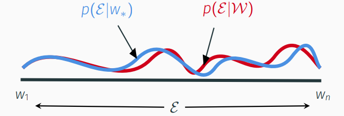
Definition: \(w_*\) paraphrases $\mathcal{W}$ if the paraphrase error \({\rho}^{\mathcal{W}, w_*}\!\in\! \mathbb{R}^{n}\) is (element-wise) small:
\[\begin{equation} {\rho}^{\mathcal{W}, w_*}_j = \log \tfrac{p(c_j|w_*)}{p(c_j|\mathcal{W})}\ , \quad c_j\!\in\!\mathcal{E}. \end{equation}\]
Paraphase error quantifies the similarity of the context distribution around any two words \(w_1, w_2\) to that of any other word \(w_*\) in terms of their PMI vectors:
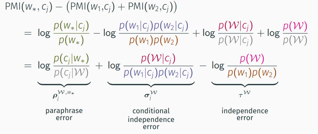
The difference comprises the paraphrase error, which is small only when \(w_*\) paraphrases \(\{w_1, w_2\}\), and dependence error terms that do not depend on $w_*$. We formalise this as:
Lemma 1: For any word \(w_*\!\in\!\mathcal{E}\) and word set \(\mathcal{W}\!\subseteq\!\mathcal{E}\), \(|\mathcal{W}|\!<\!l\), where \(l\) is the context window size:
\[\begin{equation} \text{PMI}_* \ =\ \sum_{w_i\in\mathcal{W}} \text{PMI}_{i} \,+\, \rho^{\mathcal{W}, w_*} \,+\, \sigma^{\mathcal{W}} \,-\, \tau^\mathcal{W}\mathbf{1}\ . \end{equation}\]
This connects paraphrasing to PMI vector addition, as appears in \eqref{eq:two}, and is readily generalised to quantify the relationship between word sets. We say \(\mathcal{W}\) and \(\mathcal{W}_*\) paraphrase one another if the distributions of context words around them are similar (this reduces to the original definition if \(\mathcal{W}_*\) contains a single word). Lemma 1 naturally extends to:
Lemma 2: For any word sets \(\mathcal{W}, \mathcal{W}_*\!\subseteq\!\mathcal{E}\); \(|\mathcal{W}|, |\mathcal{W}_*|\!<\!l\):
\[\begin{equation} \sum_{w_i\in\mathcal{W}_*} \text{PMI}_{i} \ =\ \sum_{w_i\in\mathcal{W}} \text{PMI}_{i} \,+\, \rho^{\mathcal{W}, \mathcal{W}_*} \,+\, (\sigma^{\mathcal{W}} - \sigma^{\mathcal{W}_*}) \,-\, (\tau^\mathcal{W} - \tau^{\mathcal{W}_*})\mathbf{1} \end{equation}\]
To see how this relates to paraphrases, let \(\mathcal{W} \!=\! \{woman, king\}\) and \(\mathcal{W}_* \!=\! \{man, queen\}\), whereby
\[\begin{equation} \text{PMI}_{king} - \text{PMI}_{man} + \text{PMI}_{woman} \ \approx\ \text{PMI}_{queen}\ , \end{equation}\]if (a) \(\mathcal{W}\) paraphrases \(\mathcal{W}_*\) (i.e. \(\rho^{\mathcal{W}, \mathcal{W}_*}\) is small) and (b) net statistical dependencies are small for words in \(\mathcal{W}\) and \(\mathcal{W}_*\) (i.e. \(\sigma^{\mathcal{W}} - \sigma^{\mathcal{W}_*}\) and \(\tau^\mathcal{W} - \tau^{\mathcal{W}_*}\)).
| Thus, subject to dependence errors, \eqref{eq:two} holds if \(\{woman, king\}\) paraphrases \(\{man, queen\}\). |
This establishes that two paraphrases are a sufficient condition for the geometric relationship between word embeddings observed for an analogy. What remains then, is to show that an analogy “\(w_a\text{ is to }w_{a^*}\text{ as }w_b\text{ is to }w_{b^*}\)” implies that \(\{w_b, w_{a^*}\!\}\) paraphrases \(\{w_a, w_{b^*}\!\}\). In fact, we show an equivalence by reinterpreting paraphrases as word transformations.
Word Transformation
The paraphrasing of a word set \(\mathcal{W}\) by a word \(w_*\) can be interpreted as a semantic equivalence between \(\mathcal{W}\) and \(w_*\), denoted \(\approx_p\). Alternatively, for a particular word $w$ in $\mathcal{W}$, a paraphrase indicates which words (the remainder of \(\mathcal{W}\), denoted \(\mathcal{W}^+\)) that, when combined with \(w\), make it “more like” – or transform it to – \(w_*\). For example, the paraphrase of \(\{man, royal\}\) by \(king\) can be viewed as a word transformation from \(man\) to \(king\) by adding \(royal\). The added words have the effect of narrowing the context or, more precisely, alter the distribution of context words around \(w\) to more closely align with that of \(w_*\). We can illustrate this as:

where the paraphrase acts as the “glue” in a relationship from \(w\) to \(w_*\). Thus, for \(w\!\in\!\mathcal{W}\) and \(\mathcal{W}^+ \!=\! \mathcal{W}\!\setminus\!\!\{w\}\), saying “\(w_*\) paraphrases \(\mathcal{W}\)” is equivalent to saying “there exists a word transformation from \(w\) to \(w_*\) by adding \(\mathcal{W}^+\)”. Nothing changes other than the perspective.
Extending this to paraphrases between word sets \(\mathcal{W}\), \(\mathcal{W}_*\!\), we can choose \(w \!\in\! \mathcal{W}\), \(w_* \!\in\! \mathcal{W}_*\) and view the paraphrase as defining a relationship between \(w\) and \(w_*\) where \(\mathcal{W}^+ \!=\! \mathcal{W}\!\setminus\!\!\{w\}\) is added to \(w\) and \(\mathcal{W}^- \!=\! \mathcal{W_*}\!\!\setminus\!\!\{w_*\}\) to \(w_*\):

This is not (yet) a word transformation, as it lacks the notion of direction from \(w\) to \(w_*\). But, rather than viewing words in \(\mathcal{W}^-\) as added to \(w_*\), we consider them subtracted from \(w\) (hence our naming convention):

Just as adding words narrows the context, subtracted words can be viewed as broadening the context.
Definition: there exists a word transformation from \(w\) to \(w_*\) with transformation parameters \(\mathcal{W}^+\), \(\mathcal{W}^-\subseteq\mathcal{E}\) iff \(\ \{w\}\!\cup\!\mathcal{W}^+ \approx_\text{P} \{w_*\}\!\cup\!\mathcal{W}^-\).
Intuition
The intuition behind word transformations mirrors simple algebra: e.g. 5 is transformed to 8 by adding 3, but if 3 were somehow unavailable, then we could add 4 and subtract 1. With paraphrases alone, words can only be added to \(w\) to transform it to \(w_*\), and perhaps no word exists to describe such “semantic difference”. With word transformations, differences between words can also be used offering a far richer toolkit, e.g. the difference between \(man\) and \(king\) might be described crudely by, say, \(royal\) or $crown$, but is perhaps better described by the difference between $woman$ and $queen$. More generally, transformation parameters (\(\mathcal{W}^+, \mathcal{W}^-\)) describe the difference between \(w\) and \(w_*\) or, one might say, how “\(w\) is to \(w_*\)”.
Interpreting Analogies
We can now mathematically interpret the language of an analogy:
Definition (analogy): ”\(w_a\) is to \(w_{a^*}\) as \(w_b\) is to \(w_{b^*}\!\)” iff there exist transformation parameters \(\mathcal{W}^+\!, \mathcal{W}^-\!\subseteq\!\mathcal{E}\) that simultaneously transform both \(w_a\) to \(w_{a^*}\) and \(w_b\) to \(w_{b^*}\).
Each occurrence of “is to” in the analogy defintion is synonymous to a set of word transformation parameters and “as” implies their equality. Intuitively, this means that the semantic difference within each word pair, as now quantified, must be the same.
So, an analogy is a pair of word transformations with common parameters \(\mathcal{W}^+, \mathcal{W}^-\), but what are those parameters? Fortunately, we need not search or guess. We show in the paper (Sec 6.4) that if an analogy holds, then any parameters that transform one of the word pairs, e.g. \(w_a\) to \(w_{a^*}\), must also transform the other pair. We can therefore choose \(\mathcal{W}^+\!=\!\{w_{a^*}\!\}\), \(\mathcal{W}^-\!=\!\{w_{a}\}\). These trivially transform \(w_a\) to \(w_{a^*}\) since \(\{w_a, w_{a^*}\!\}\) exactly paraphrases \(\{w_{a^*\!}, w_a\}\) (word order is irrelevant). For the analogy to hold, those parameters must then also transform \(w_b\) to \(w_{b^*}\), i.e. \(\{w_b, w_{a^*}\}\) paraphrases \(\{w_{b^*}, w_a\}\), that is:
\[\begin{equation} w_a \text{ is to } w_{a^*} \text{ as } w_b \text{ is to } w_{b^*}\!\!" \quad\iff\quad \{w_b, w_{a^*}\} \approx_\text{P} \{w_{b^*}, w_a\}. \tag{3}\label{eq:three} \end{equation}\]This completes the chain:
- analogies are equivalent to word transformations with common transformation parameters describing a common “semantic difference” \eqref{eq:three};
- those word transformations define a readily identifiable paraphrase;
- that paraphrase implies a geometric relationship between PMI vectors \eqref{eq:two} that depends on the paraphrase accuracy (\(\rho\)) and dependence error terms (\(\sigma, \tau\)); and
- under a low-dimensional projection induced by the loss function, that geometric relationship is reflected between the word embeddings of an analogy \eqref{eq:one}.
Returning to an initial plot, we can now explain the “gap” in terms of paraphrase (\(\rho\)) and dependence \((\sigma, \tau\)) error terms, and understand why it is variable but often smallest for words that complete the analogy. This concludes an end-to-end explanation for the geometric relationship between word embeddings observed for word analogies.
Extensions
- “What the Vec? Towards Probabilistically Grounded Embeddings” extends the principles of this work to show: how W2V and Glove (approximately) capture other relationships such as relatedness and similarity; what certain embedding interactions correspond to; and, in doing so, how the semantic relationships of relatedness, similarity, paraphrasing and analogies mathematically inter-relate.
- “Multi-relational Poincaré Graph Embeddings” [code] draws a comparison between analogies and relations in Knowledge Graphs to develop state-of-the-art representation models in both Euclidean and Hyperbolic space.
Related Work
Several other works aim to theoretically explain the analogy phenomenon, in particular:
- Arora et al. (2016) propose a latent variable model for text generation that is claimed inter alia to explain analogies, however strong a priori assumptions are made about the arrangement of word vectors that we do not require.
- Gittens et al. (2017) introduce the idea of paraphrasing to explain analogies, from which we drew much inspiration, but they include several assumptions that fail in practice, in particular that word frequencies follow a uniform distribution rather than their true, highly non-uniform, Zipf distribution.
- Ethayarajh et al. (2019) aim to show that word embeddings of analogies form parallelograms by considering the latter’s geometric properties. However, several strong assumptions are made that we do not require (e.g. all embedding must already be co-planar and embedding matrix \(\mathbf{W}\) must be a scalar multiple of \(\mathbf{C}\)) and analogies are ultimately related to a statistical relationship “csPMI” that lacks semantic meaning.